Tutorial
Note
This tutorial is available as an IPython notebook here.
%matplotlib inline
import matplotlib.pyplot as plt
plt.style.use('ggplot')
from itertools import chain

import nltk
import sklearn
import scipy.stats
from sklearn.metrics import make_scorer
from sklearn.cross_validation import cross_val_score
from sklearn.grid_search import RandomizedSearchCV

import sklearn_crfsuite
from sklearn_crfsuite import scorers
from sklearn_crfsuite import metrics
Let’s use CoNLL 2002 data to build a NER system
CoNLL2002 corpus is available in NLTK. We use Spanish data.
nltk.corpus.conll2002.fileids()
['esp.testa', 'esp.testb', 'esp.train', 'ned.testa', 'ned.testb', 'ned.train']
%%time
train_sents = list(nltk.corpus.conll2002.iob_sents('esp.train'))
test_sents = list(nltk.corpus.conll2002.iob_sents('esp.testb'))
CPU times: user 2.91 s, sys: 108 ms, total: 3.02 s
Wall time: 3.13 s
train_sents[0]
[('Melbourne', 'NP', 'B-LOC'),
 ('(', 'Fpa', 'O'),
 ('Australia', 'NP', 'B-LOC'),
 (')', 'Fpt', 'O'),
 (',', 'Fc', 'O'),
 ('25', 'Z', 'O'),
 ('may', 'NC', 'O'),
 ('(', 'Fpa', 'O'),
 ('EFE', 'NC', 'B-ORG'),
 (')', 'Fpt', 'O'),
 ('.', 'Fp', 'O')]
Features
Next, define some features. In this example we use word identity, word suffix, word shape and word POS tag; also, some information from nearby words is used.
This makes a simple baseline, but you certainly can add and remove some features to get (much?) better results - experiment with it.
sklearn-crfsuite (and python-crfsuite) supports several feature formats; here we use feature dicts.
def word2features(sent, i):
    word = sent[i][0]
    postag = sent[i][1]

    features = {
        'bias': 1.0,
        'word.lower()': word.lower(),
        'word[-3:]': word[-3:],
        'word[-2:]': word[-2:],
        'word.isupper()': word.isupper(),
        'word.istitle()': word.istitle(),
        'word.isdigit()': word.isdigit(),
        'postag': postag,
        'postag[:2]': postag[:2],
    }
    if i > 0:
        word1 = sent[i-1][0]
        postag1 = sent[i-1][1]
        features.update({
            '-1:word.lower()': word1.lower(),
            '-1:word.istitle()': word1.istitle(),
            '-1:word.isupper()': word1.isupper(),
            '-1:postag': postag1,
            '-1:postag[:2]': postag1[:2],
        })
    else:
        features['BOS'] = True

    if i < len(sent)-1:
        word1 = sent[i+1][0]
        postag1 = sent[i+1][1]
        features.update({
            '+1:word.lower()': word1.lower(),
            '+1:word.istitle()': word1.istitle(),
            '+1:word.isupper()': word1.isupper(),
            '+1:postag': postag1,
            '+1:postag[:2]': postag1[:2],
        })
    else:
        features['EOS'] = True

    return features


def sent2features(sent):
    return [word2features(sent, i) for i in range(len(sent))]

def sent2labels(sent):
    return [label for token, postag, label in sent]

def sent2tokens(sent):
    return [token for token, postag, label in sent]
This is what word2features extracts:
sent2features(train_sents[0])[0]
{'+1:postag': 'Fpa',
 '+1:postag[:2]': 'Fp',
 '+1:word.istitle()': False,
 '+1:word.isupper()': False,
 '+1:word.lower()': '(',
 'BOS': True,
 'bias': 1.0,
 'postag': 'NP',
 'postag[:2]': 'NP',
 'word.isdigit()': False,
 'word.istitle()': True,
 'word.isupper()': False,
 'word.lower()': 'melbourne',
 'word[-2:]': 'ne',
 'word[-3:]': 'rne'}
Extract features from the data:
%%time
X_train = [sent2features(s) for s in train_sents]
y_train = [sent2labels(s) for s in train_sents]

X_test = [sent2features(s) for s in test_sents]
y_test = [sent2labels(s) for s in test_sents]
CPU times: user 1.48 s, sys: 124 ms, total: 1.61 s
Wall time: 1.65 s
Training
To see all possible CRF parameters check its docstring. Here we are useing L-BFGS training algorithm (it is default) with Elastic Net (L1 + L2) regularization.
%%time
crf = sklearn_crfsuite.CRF(
    algorithm='lbfgs',
    c1=0.1,
    c2=0.1,
    max_iterations=100,
    all_possible_transitions=True
)
crf.fit(X_train, y_train)
CPU times: user 32 s, sys: 108 ms, total: 32.1 s
Wall time: 32.3 s
Evaluation
There is much more O entities in data set, but we’re more interested in
other entities. To account for this we’ll use averaged F1 score computed
for all labels except for O. sklearn-crfsuite.metrics package
provides some useful metrics for sequence classification task, including
this one.
labels = list(crf.classes_)
labels.remove('O')
labels
['B-LOC', 'B-ORG', 'B-PER', 'I-PER', 'B-MISC', 'I-ORG', 'I-LOC', 'I-MISC']
y_pred = crf.predict(X_test)
metrics.flat_f1_score(y_test, y_pred,
                      average='weighted', labels=labels)
0.76980231377134023
Inspect per-class results in more detail:
# group B and I results
sorted_labels = sorted(
    labels,
    key=lambda name: (name[1:], name[0])
)
print(metrics.flat_classification_report(
    y_test, y_pred, labels=sorted_labels, digits=3
))
             precision    recall  f1-score   support

      B-LOC      0.775     0.757     0.766      1084
      I-LOC      0.601     0.631     0.616       325
     B-MISC      0.698     0.499     0.582       339
     I-MISC      0.644     0.567     0.603       557
      B-ORG      0.795     0.801     0.798      1400
      I-ORG      0.831     0.773     0.801      1104
      B-PER      0.812     0.876     0.843       735
      I-PER      0.873     0.931     0.901       634

avg / total      0.779     0.764     0.770      6178
Hyperparameter Optimization
To improve quality try to select regularization parameters using randomized search and 3-fold cross-validation.
I takes quite a lot of CPU time and RAM (we’re fitting a model
50 * 3 = 150 times), so grab a tea and be patient, or reduce n_iter
in RandomizedSearchCV, or fit model only on a subset of training data.
%%time
# define fixed parameters and parameters to search
crf = sklearn_crfsuite.CRF(
    algorithm='lbfgs',
    max_iterations=100,
    all_possible_transitions=True
)
params_space = {
    'c1': scipy.stats.expon(scale=0.5),
    'c2': scipy.stats.expon(scale=0.05),
}

# use the same metric for evaluation
f1_scorer = make_scorer(metrics.flat_f1_score,
                        average='weighted', labels=labels)

# search
rs = RandomizedSearchCV(crf, params_space,
                        cv=3,
                        verbose=1,
                        n_jobs=-1,
                        n_iter=50,
                        scoring=f1_scorer)
rs.fit(X_train, y_train)
Fitting 3 folds for each of 50 candidates, totalling 150 fits
[Parallel(n_jobs=-1)]: Done  34 tasks      | elapsed:  4.1min
[Parallel(n_jobs=-1)]: Done 150 out of 150 | elapsed: 16.1min finished
CPU times: user 3min 34s, sys: 13.9 s, total: 3min 48s
Wall time: 16min 36s
Best result:
# crf = rs.best_estimator_
print('best params:', rs.best_params_)
print('best CV score:', rs.best_score_)
print('model size: {:0.2f}M'.format(rs.best_estimator_.size_ / 1000000))
best params: {'c2': 0.06146442424219609, 'c1': 0.30343585910230675}
best CV score: 0.748852160441
model size: 1.08M
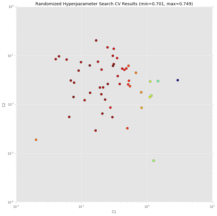
Check parameter space
A chart which shows which c1 and c2 values have
RandomizedSearchCV checked. Red color means better results, blue means
worse.
_x = [s.parameters['c1'] for s in rs.grid_scores_]
_y = [s.parameters['c2'] for s in rs.grid_scores_]
_c = [s.mean_validation_score for s in rs.grid_scores_]

fig = plt.figure()
fig.set_size_inches(12, 12)
ax = plt.gca()
ax.set_yscale('log')
ax.set_xscale('log')
ax.set_xlabel('C1')
ax.set_ylabel('C2')
ax.set_title("Randomized Hyperparameter Search CV Results (min={:0.3}, max={:0.3})".format(
    min(_c), max(_c)
))

ax.scatter(_x, _y, c=_c, s=60, alpha=0.9, edgecolors=[0,0,0])

print("Dark blue => {:0.4}, dark red => {:0.4}".format(min(_c), max(_c)))
Dark blue => 0.7013, dark red => 0.7489
Check best estimator on our test data
As you can see, quality is improved.
crf = rs.best_estimator_
y_pred = crf.predict(X_test)
print(metrics.flat_classification_report(
    y_test, y_pred, labels=sorted_labels, digits=3
))
             precision    recall  f1-score   support

      B-LOC      0.800     0.780     0.790      1084
      I-LOC      0.663     0.625     0.643       325
     B-MISC      0.729     0.555     0.630       339
     I-MISC      0.709     0.582     0.639       557
      B-ORG      0.808     0.824     0.816      1400
      I-ORG      0.849     0.783     0.814      1104
      B-PER      0.836     0.882     0.858       735
      I-PER      0.884     0.942     0.912       634

avg / total      0.804     0.781     0.791      6178
Let’s check what classifier learned
from collections import Counter

def print_transitions(trans_features):
    for (label_from, label_to), weight in trans_features:
        print("%-6s -> %-7s %0.6f" % (label_from, label_to, weight))

print("Top likely transitions:")
print_transitions(Counter(crf.transition_features_).most_common(20))

print("\nTop unlikely transitions:")
print_transitions(Counter(crf.transition_features_).most_common()[-20:])
Top likely transitions:
B-ORG  -> I-ORG   7.029925
I-ORG  -> I-ORG   6.672091
B-MISC -> I-MISC  6.450077
I-MISC -> I-MISC  6.420227
B-PER  -> I-PER   5.898448
B-LOC  -> I-LOC   5.293131
I-LOC  -> I-LOC   4.669233
I-PER  -> I-PER   4.327948
O      -> O       3.773498
O      -> B-ORG   2.723333
O      -> B-PER   2.298990
O      -> B-LOC   1.753950
O      -> B-MISC  1.608865
B-ORG  -> O       0.373792
B-LOC  -> B-LOC   0.363950
B-MISC -> B-ORG   0.213808
B-ORG  -> B-LOC   0.122352
I-PER  -> B-LOC   0.055117
B-LOC  -> B-PER   -0.141696
B-MISC -> O       -0.170980

Top unlikely transitions:
I-ORG  -> B-LOC   -2.281004
I-LOC  -> I-PER   -2.285589
I-MISC -> B-LOC   -2.286738
I-LOC  -> B-MISC  -2.299090
B-LOC  -> B-MISC  -2.312090
I-ORG  -> I-PER   -2.636941
I-ORG  -> B-MISC  -2.673906
B-ORG  -> B-MISC  -2.735029
I-PER  -> B-ORG   -2.822961
B-PER  -> B-MISC  -2.857271
I-MISC -> I-LOC   -2.902497
I-PER  -> I-LOC   -2.931078
I-ORG  -> I-LOC   -2.943800
B-PER  -> B-PER   -3.063315
I-PER  -> B-MISC  -3.373836
B-MISC -> B-MISC  -3.435245
O      -> I-MISC  -5.385205
O      -> I-ORG   -5.670565
O      -> I-PER   -6.003255
O      -> I-LOC   -6.680094
We can see that, for example, it is very likely that the beginning of an organization name (B-ORG) will be followed by a token inside organization name (I-ORG), but transitions to I-ORG from tokens with other labels are penalized.
Check the state features:
def print_state_features(state_features):
    for (attr, label), weight in state_features:
        print("%0.6f %-8s %s" % (weight, label, attr))

print("Top positive:")
print_state_features(Counter(crf.state_features_).most_common(30))

print("\nTop negative:")
print_state_features(Counter(crf.state_features_).most_common()[-30:])
Top positive:
11.005266 B-ORG    word.lower():efe-cantabria
9.385823 B-ORG    word.lower():psoe-progresistas
6.715219 I-ORG    -1:word.lower():l
5.638921 O        BOS
5.378117 B-LOC    -1:word.lower():cantabria
5.302705 B-ORG    word.lower():xfera
5.287491 B-ORG    word[-2:]:-e
5.239806 B-ORG    word.lower():petrobras
5.214013 B-MISC   word.lower():diversia
5.025534 B-ORG    word.lower():coag-extremadura
5.020590 B-ORG    word.lower():telefónica
4.804399 B-MISC   word.lower():justicia
4.729711 B-MISC   word.lower():competencia
4.705013 O        postag[:2]:Fp
4.695208 B-ORG    -1:word.lower():distancia
4.681021 I-ORG    -1:word.lower():rasd
4.636151 I-LOC    -1:word.lower():calle
4.618459 B-ORG    word.lower():terra
4.580418 B-PER    -1:word.lower():según
4.574348 B-ORG    word.lower():esquerra
4.537127 O        word.lower():r.
4.537127 O        word[-3:]:R.
4.536578 B-MISC   word.lower():cc2305001730
4.510408 B-ORG    +1:word.lower():plasencia
4.471889 B-LOC    +1:word.lower():finalizaron
4.451102 B-LOC    word.lower():líbano
4.423293 B-ORG    word.isupper()
4.379665 O        word.lower():euro
4.361340 B-LOC    -1:word.lower():celebrarán
4.345542 I-MISC   -1:word.lower():1.9

Top negative:
-2.006512 I-PER    word[-3:]:ión
-2.020133 B-PER    word[-2:]:os
-2.027996 O        +1:word.lower():campo
-2.028221 O        +1:word.lower():plasencia
-2.043293 O        word.lower():061
-2.097561 O        postag:NP
-2.097561 O        postag[:2]:NP
-2.115992 O        word[-3:]:730
-2.156136 O        word.lower():circo
-2.173247 B-LOC    word[-3:]:la
-2.223739 I-PER    +1:word.lower():del
-2.323688 B-MISC   -1:word.isupper()
-2.347859 O        -1:word.lower():sánchez
-2.378442 I-PER    word[-3:]:ico
-2.404641 I-PER    +1:word.lower():el
-2.414000 O        word[-3:]:bas
-2.495209 O        -1:word.lower():británica
-2.539839 B-PER    word[-3:]:nes
-2.596765 O        +1:word.lower():justicia
-2.621004 O        -1:word.lower():sección
-2.981810 O        word[-3:]:LOS
-3.046486 O        word[-2:]:nd
-3.162064 O        -1:word.lower():españolas
-3.219096 I-PER    -1:word.lower():san
-3.562049 B-PER    -1:word.lower():del
-3.580405 O        word.lower():mas
-4.119731 O        word[-2:]:om
-4.301704 O        -1:word.lower():celebrarán
-5.632036 O        word.isupper()
-8.215073 O        word.istitle()
Some observations:
- 9.385823 B-ORG word.lower():psoe-progresistas - the model remembered names of some entities - maybe it is overfit, or maybe our features are not adequate, or maybe remembering is indeed helpful;
- 4.636151 I-LOC -1:word.lower():calle: “calle” is a street in Spanish; model learns that if a previous word was “calle” then the token is likely a part of location;
- -5.632036 O word.isupper(), -8.215073 O word.istitle() : UPPERCASED or TitleCased words are likely entities of some kind;
- -2.097561 O postag:NP - proper nouns (NP is a proper noun in the Spanish tagset) are often entities.
What to do next
* Load 'testa' Spanish data.
* Use it to develop better features and to find best model parameters.
* Apply the model to 'testb' data again.
The model in this notebook is just a starting point; you certainly can do better!